EVE Online: Jita to Amarr

EVE Online is a fun, and possibly psychotic MMORPG that takes place in an expansive stellar cluster with some truly mind-boggling distances involved. To fully explore this universe you can expect to spend over 9 years of your life.

In a game where logistics and industry make news-worth battles possible, calculating optimal routes between systems and stations becomes an important task.

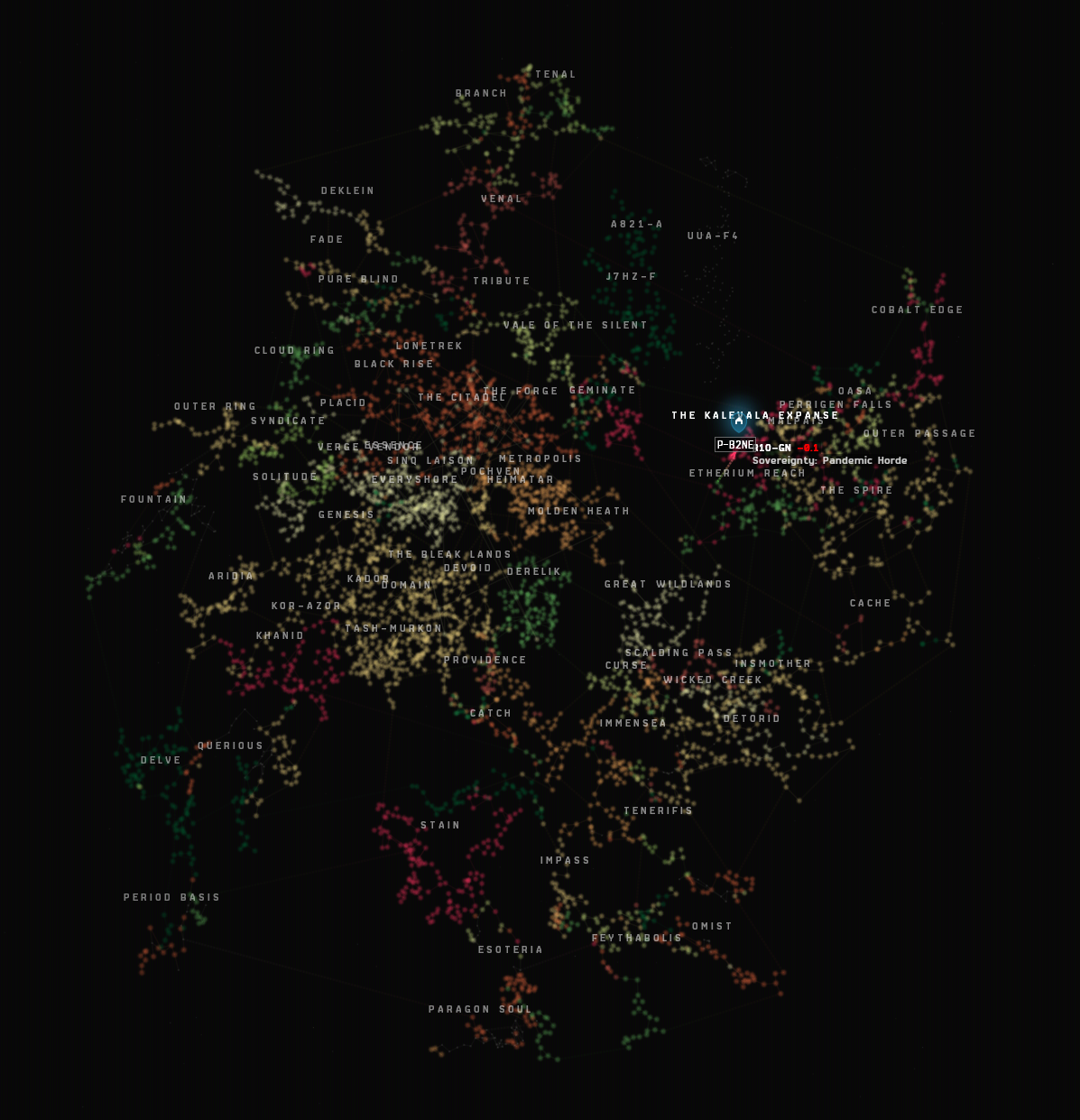
Taking our first look at the EVE Universe can be a little daunting. A total of 8285 stars make up the stellar cluster, although not all of them are player-accessible. A few, known as wormholes or J-space, are not permanently attached to any part of the map and their connections roam around. The remaining systems that are permanently connected to each other make up what is known as k-space, or known-space. 13753 stargates form the permanent connection points between the stars. Let's take another look, this time from a top-down, abstract view:

If you've ever done graph theory, this probably looks pretty familiar. The EVE universe can be ideally represented as a simple graph. Each solar system is a vertex (or node), in the graph, and each pair of stargates forms an edge between two vertices.

We're going to use Python to create a graph we can use to answer simple questions like "What's the shortest route to get from Jita to Amarr". Later, we'll make it a bit more complex so we can add new conditions, like finding the safest route. In the actual tool this article is based off of, we pull the systems and stargates from EVE's API, known as the ESI, but to keep things simple you can simply download these two JSON files, which contain all the systems and stargates.

• systems.json
• stargates.json

There are several popular libraries for working with graphs in Python, such as networkx and igraph. Networkx is a native python library that trades intuitive usage, flexible types and good error messages for high memory usage and slower speed. igraph is a C library with python bindings that is harder to use and less intuitive, but offers significantly better memory usage and faster lookups. For this article, we want simple, so we're sticking with networkx.

Our first step is to load the data. Remember, our systems are our nodes, and the connections between stargates form our edges:

import json
import networkx as nx

graph = nx.Graph()

with open('systems.json', 'rb') as systems_json:
    systems = json.load(systems_json)

    for system in systems:
        graph.add_node(system['system_id'], name=system['name'])

graph.add_node() takes a unique identifier for the node and any extra attributes we want to save on it, in this case the name of the system. One nice thing we get from networkx is the ability to use our system's IDs as the node ID. In igraph, we get incremental numbers as our node IDs. Now that we have all the systems added, we're going to add the edges:

with open('stargates.json', 'rb') as stargates_json:
    stargates = json.load(stargates_json)

    for stargate in stargates:
        graph.add_edge(
            stargate['system_id'],
            stargate['destination_system_id']
        )

We're actually done here. We can answer our original question of "What's the shortest route to get from Jita to Amarr" with what we've done already:

print(
   nx.shortest_path(
        graph,
        30000142, # The System ID for Jita
        30002187  # The System ID for Amarr
    )
)
[30000142, 30000138, 30000132, 30000134, 30005196, 30005192,
    30004083, 30004078, 30004079, 30004080, 30002282, 30002187]

Those numbers are the systems IDs we'd need to pass through to get from Jita to Amarr in the shortest possible distance, and we got the answer in less than a millisecond. Not very useful on their own, but we could easily look up the names from the systems.json file we loaded earlier.

When we called nx.shortest_path(), networkx used an algorithm called Dijkstra's algorithm to efficiently find the shortest path between Jita (30000142) and Amarr (30002187). It's actually a very simple algorithm, and if you don't want to use networkx you could implement it yourself pretty quickly.

Not all roads are worth taking

Just because a route is the shortest on paper doesn't mean it's the best route to take. Walking over a mountain is rarely faster than walking around it. In EVE, the relative safety of a system is represented as a value known a its "security status", which is a number with 3 ranges:

Remember that short 11-jump route we found earlier? You would probably have died 4 jumps in as that system is low-sec, allowing other players to attack you with minimal repercussions.

["Jita", 30000138, 30000132, 30000134, "DEATH", 30005192,
    30004083, 30004078, 30004079, 30004080, 30002282, "Amarr"]

If you never make it to your destination, it's not really the shortest route now, is it? We're going to fix this by adding some more information to our graph. Let's go back to where we loaded up nodes and edges and make a few changes:

import json
import networkx as nx

graph = nx.MultiDiGraph()

with open('systems.json', 'rb') as systems_json:
    systems = {
        system['system_id']: system
        for system in json.load(systems_json)
    }

with open('stargates.json', 'rb') as stargates_json:
    stargates = json.load(stargates_json)


for system_id, system in systems.items():
    graph.add_node(system_id, name=system['name'])


for stargate in stargates:
    security = systems[stargate['destination_system_id']]['security_status']

    graph.add_edge(
        stargate['system_id'],
        stargate['destination_system_id'],
        ls=0 if security < 0.45 else 1,
        hs=0 if security >= 0.45 else 1
    )

Right away you should notice a few things. Our graph is no longer a nx.Graph(), it's now a nx.MultiDiGraph(). This is important! Our original graph didn't have a concept of direction, and didn't allow multiple edges between the same nodes. We've also stored two attributes on each edge, hs (high-security) and ls (low-security), which are weights we'll use later to determine if we should take this edge when looking for safe or unsafe paths.

So why have we changed the type of graph we're making? If we sketched our original graph two connected systems would look something like this:

Then we add direction, turning our graph into a directed graph:

Then we add the return paths, turning our graph into a directed graph with multiple edges, or a MultiDiGraph() in networkx:

Now our graph has all the information we need to pick a much safer route. Let's try our shortest path between Jita and Amarr again:

nx.shortest_path(
    graph,
    30000142, # The System ID for Jita
    30002187, # The System ID for Amarr
    weight='hs' # Use the 'hs' attribute for weights
)
[30000142, 30000144, 30000139, 30002802, 30002801, 30002803, 30002768,
 30002765, 30002764, 30002761, 30004972, 30004970, 30002633, 30002634,
 30002641, 30002681, 30002682, 30002048, 30002049, 30002053, 30002543,
 30002544, 30002568, 30002529, 30002530, 30002507, 30002509, 30000004,
 30000005, 30000002, 30002973, 30002969, 30002974, 30002972, 30002971,
 30002970, 30002963, 30002964, 30002991, 30002994, 30003545, 30003548,
 30003525, 30003523, 30003522, 30002187]

That's quite a bit longer, at 46 jumps! However, we're more likely to actually arrive at our destination by taking a route through safer systems.

Note that we've simply done safe or unsafe here. Instead of a 0 or a 1, we could have scaled the weight by how safe the system was. We could also mix in other values, such as "Has someone died here recently?"

Sometimes you want to stay in the less-secure systems. If you're a criminal, you don't want to run into the police now, do you? We would simply use weight='ls' to get a route that we keep us in less-secure space.

Space and Time

There's actually two different routes with the same number of jumps between Jita and Amarr:

[30000142, 30000138, 30000132, 30000134, 30005196, 30005192, 30004083,
 30004078, 30004079, 30004080, 30002282, 30002187]
[30000142, 30000138, 30000132, 30000134, 30005196, 30005192, 30004083,
 30004081, 30002197, 30002193, 30003491, 30002187]

These routes show a fork in the road at jump 8, which rejoin at the same system at jump 11. We could add some extra information to our graph to prefer the route that is also physically the shortest number of lightyears across which would be very helpful for slow ships in EVE like the big hulking freighters.

On very long routes its more likely you'll have multiple routes with the same length, and over really long distances you'll sometimes run into situations where taking an extra system is actually faster due to how far apart the stargates are within a system. It's also simply convenient knowing how long your trip will take.

There's a lot of ways to answer this question, but in the spirit of this article we're going to use an even bigger graph. We're going to add all the stargates we know about to the graph as nodes, and create edges between them, storing the distance between any two nodes in a system as an attribute on the edges between them.

This graph combines everything we've done so far. Our edges between linked stargates know the security status of the destination, letting us avoid unsafe systems. Our edges between locations within a system know the distance between them, letting us sum the total distance travelled.

In practice, this graph will be much messier to visualize. You wouldn't just include the star and the stargates, but the planets, moons, asteroid belts, stations, citadels, player-owned-stations (POS), and anything else with a static position in the system. We don't really care about being exact, we just want approximate times, so we're fine with using the star in the center of the system as our starting position whenever we're unsure of where the user is starting their journey.

We leave the rest as an exercise to the reader, but you see how the simple graph we started with can be expanded to cover quite a few different cases using the same simple algorithms.